As a PIM company, we understand the limitations of spreadsheets when it comes to managing complex product data. However, we also know that spreadsheets can be a useful tool for preparing data for a PIM system. Our team of experts at OneTimePIM has extensive experience handling product data for companies across various industries, and we are always looking for ways to improve and streamline our processes.
In this article, we have compiled a list of 6 clever spreadsheet formulas that our experts use regularly to manage product information. Whether you are already using these formulas or are new to them, we believe they can help you optimize your data management processes and save time.
VLOOKUP
VLOOKUP is a function in Microsoft Excel that allows you to find and retrieve data from a table based on a specific search term. This function is useful for quickly locating a data point that would otherwise require manual scrolling and searching through a large spreadsheet. For example, if you are managing product information, you may need to quickly find the price for a certain part code.
To use VLOOKUP, you first select the cell where you want the retrieved data to appear and type =VLOOKUP(). Then, inside the parentheses, you provide four pieces of information separated by commas: the search term (i.e., the data point you already know), the table range to search within, the column number in the table that contains the desired data, and the word "FALSE" to indicate an exact match.
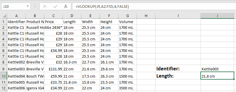
For example, if you want to find the length associated with the identifier "Kettle005," you might enter the following formula into a cell:
=VLOOKUP("Kettle005", A2:F55, 4, FALSE)
This formula would search the range of cells A2 through F55, look for the value "Kettle005" in the first column of that range, and return the value in the fourth column of that range (which, in this example, contains the length associated with the identifier).
Overall, VLOOKUP is a powerful tool for quickly finding specific data points in large spreadsheets.
CONCAT
The CONCAT function, previously known as CONCATENATE, is a useful tool in Microsoft Excel that allows you to combine data from different cells. This can be particularly helpful if you want to combine two or more pieces of information to create a unique identifier, such as an SKU number.
To use CONCAT, first select the cell where you want the combined data to appear and type =CONCAT() in the formula bar. Within the parentheses, list all the cells containing the data you want to combine, separated by commas. For example, if you want to combine the data in cells A4 and A6, you would enter =CONCAT(A4, A6).
Excel will then combine the values in the cells you have listed, with no spaces or punctuation between them. If you want to add a space, punctuation, or any other character between the combined data, you can include it as a string within quotes. For example, if you want to include a hyphen between the values in cells A4 and A6, you would enter =CONCAT(A4, "-", A6).
Overall, the CONCAT function is a helpful way to quickly combine data from different cells in Excel. It can save time and reduce errors by eliminating the need to manually enter data into a new cell.
UPPER / LOWER / PROPER
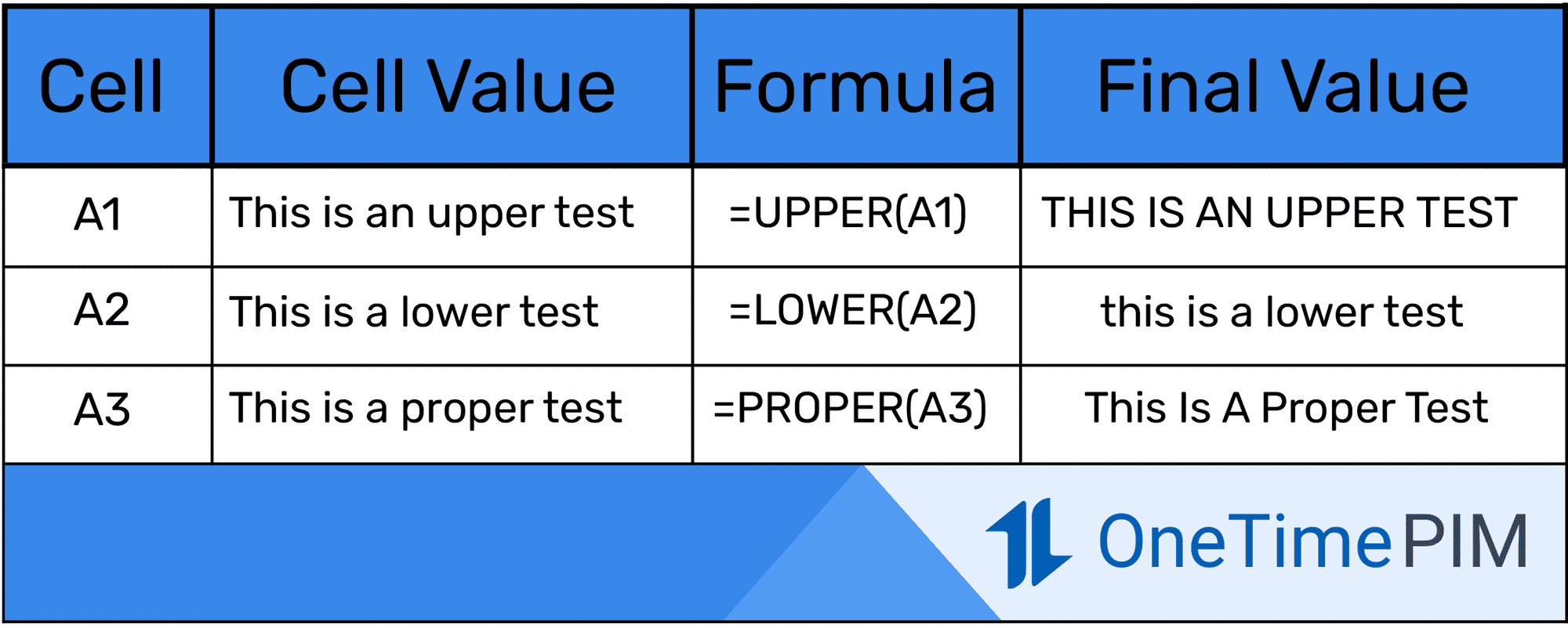
The UPPER, LOWER, and PROPER functions in Microsoft Excel allow you to change the case of letters in a cell. The UPPER function will make all the text in a cell capitalized, the LOWER function will make it all lowercase, and the PROPER function will capitalize the first letter of every word. These functions can be especially useful when generating attribute or category titles in a data sheet.
To use the UPPER, LOWER, or PROPER function, first select the cell where you want the modified data to appear. Next, type the function name (UPPER, LOWER, or PROPER) with an equals sign (=) before it, and parentheses () after it. Within the parentheses, enter the cell that you want to change the case of.
For example, if you want to make the text in cell A1 all uppercase, you would enter the following formula in another cell:
=UPPER(A1)
If you want to make the text in cell A1 all lowercase, you would use the LOWER function instead:
=LOWER(A1)
And if you want to capitalize the first letter of every word in cell A1, you would use the PROPER function:
=PROPER(A1)
After entering the formula, hit enter and the modified text will appear in the cell you selected.
In summary, the UPPER, LOWER, and PROPER functions in Excel are helpful for changing the case of letters in a cell and can be used to quickly modify text in a spreadsheet.
ISBLANK
The ISBLANK function in Microsoft Excel checks whether a specific cell is blank and returns a TRUE or FALSE message. It is often used as part of a larger nested formula, such as "if a cell is blank, then add a certain value to it."
It is important to note that cells will not be considered blank if they contain a formula, even if the formula does not display any data. Additionally, cells with only a space in them will also be considered not blank, which can be misleading.
One useful application of the ISBLANK function is when used alongside the CONCAT function. In this case, Excel can check for blank cells and fill them with data from other cells to form a complete description or title.
To use the ISBLANK function, select the cell where you want the modified data to appear, and type =ISBLANK() in the formula bar. Inside the parentheses, enter the cell that you want to check for blankness. For example, if you want to check whether cell A1 is blank, you would enter =ISBLANK(A1).
Excel will then return a TRUE or FALSE value in the cell where you entered the formula, depending on whether the selected cell contains any value.
Overall, the ISBLANK function in Excel is a helpful tool for checking if a cell is empty, and can be used in combination with other functions to manipulate data in a spreadsheet.
LEN
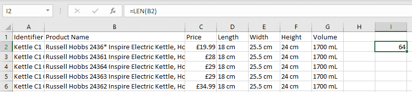
The LEN function in Microsoft Excel allows you to count the number of characters in a selected cell. This can be useful in situations where you need to limit the length of text, such as for a website description, or if you want to verify the length of data before importing it into another system.
To use the LEN function, select the cell where you want the character count to appear, and type =LEN() in the formula bar. Inside the parentheses, enter the cell that you want to count the characters for. For example, if you want to count the characters in cell A1, you would enter =LEN(A1).
Excel will then return a number indicating the amount of characters in the selected cell. It is important to note that the LEN function counts all characters, including spaces and punctuation.
Overall, the LEN function is a useful tool for quickly counting the number of characters in a cell, which can help ensure that text meets a specified length requirement. It can also be used in combination with other functions to manipulate text in a spreadsheet.
TRIM
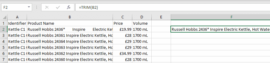
The TRIM function in Microsoft Excel removes excess spaces from text in a cell, leaving only one space between words. This can be helpful for cleaning up data and fixing errors, particularly when working with a large number of SKUs or other product information.
To use TRIM, select the cell where you want the modified data to appear, and type =TRIM() in the formula bar. Inside the parentheses, enter the cell that you want to trim off the excess spaces. For example, if you want to trim the excess spaces from cell A1, you would enter =TRIM(A1).
Excel will then remove all extra spaces, including those at the start and end of the cell, leaving only one space between words.
It is important to note that TRIM only removes spaces, so it will not remove other non-printable characters, such as tabs or line breaks. If you want to remove these characters as well, you can use the CLEAN function in combination with TRIM.
Overall, the TRIM function in Excel is a useful tool for cleaning up data and ensuring consistent formatting, particularly when working with large amounts of text.
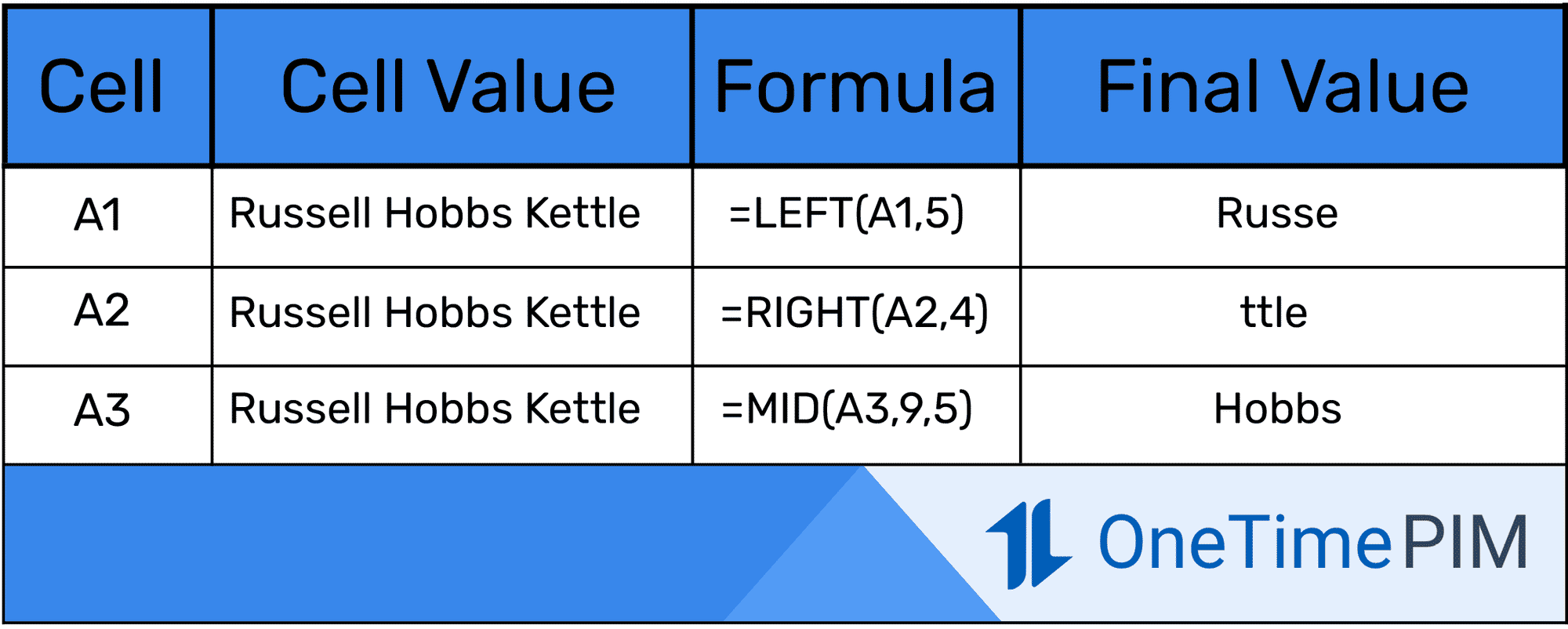
LEFT / RIGHT / MID
The LEFT, RIGHT, and MID functions in Microsoft Excel allow you to extract characters from the left, right, or middle of a cell. These functions can be especially helpful when working with large amounts of data, such as generating SKU numbers based on product names.
To use LEFT, RIGHT, or MID, select the cell where you want the modified data to appear, and type the relevant function name (LEFT, RIGHT, or MID) with an equals sign (=) before it, followed by parentheses (). Within the parentheses, enter the cell that you want to extract data from, followed by a comma.
If you are using the LEFT or RIGHT function, enter the number of characters you want to copy across after the comma, and then hit enter. For example, if you want to copy the first 3 characters of cell A1 using the LEFT function, you would enter =LEFT(A1,3).
If you are using the MID function, enter the character number you want the copying to start from, followed by a comma. Then enter the number of characters you want to copy after the second comma, and hit enter. For example, if you want to copy 4 characters starting from the second character of cell A1, you would enter =MID(A1,2,4).
Excel will then display the extracted characters in the required cell, based on the conditions you specified in the formula.
Overall, the LEFT, RIGHT, and MID functions in Excel are useful for extracting specific parts of text from cells and can be used in combination with other functions to manipulate data in a spreadsheet.
Summary
These formulas are a great tool for managing product information in Excel and can help streamline data processing for businesses. They have been carefully chosen by our expert data team, who use Excel on a daily basis in conjunction with our spreadsheet view in OneTimePIM to take advantage of the powerful benefits of both systems.
If you are struggling with data management or feel like your product data is ready for a PIM system, we would love to hear from you. Our team of experts can help guide you through the process of cleaning and organizing your data, as well as provide you with solutions for more efficient data management. With OneTimePIM, you can simplify and streamline your product data management, saving time and resources for your business.
Don't hesitate to get in touch to learn more about our PIM solutions and how we can help your business succeed.